Why does Python automatically exit a script when it’s done?
First, from your bash terminal in your PowerShell open a new file called “input.py”
nano input.py
Then paste the following into the shell by right-clicking on the PowerShell window
name=input("Don't type anything!\n")
print("Hi,",name,"!")
Now, press CTRL+X to save and exit the nano window and in your shell type:
python3 input.py
Don't type anything!
And press CTRL+D to terminate the program while it’s waiting for user input
Traceback (most recent call last):
File "input.py", line 1, in
name=input("Don't type anything!")
EOFError
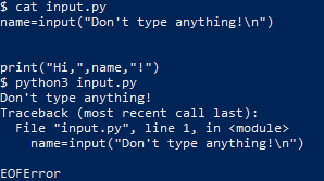
The EOFError exception tells us that the Python interpreter hit the end of file (EOF) condition before it finished executing the code, as the user entered no input data.
When Python reaches the EOF condition at the same time that it has executed all the code it exits without throwing any exceptions which is one way Python may exit “gracefully.”
Detect script exit
If we want to tell when a Python program exits without throwing an exception, we can use the built-in Python atexit module.
Theatexit handles anything we want the program to do when it exits and is typically used to do program clean up before the program process terminates
To experiment with atexit, let’s modify our input.py example to print a message at the program exit. Open the input.py file again and replace the text with this
import atexit
atexit.register(print,"Program exited successfully!")
name=input("What's your name?\n")
print("Hi,",name,"!")
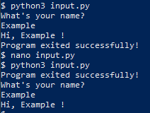
Type your name and when you hit enter you should get:
What's your name?
Example
Hi, Example !
Program exited successfully!
Notice how the exit text appears at the end of the output no matter where we place the atexit call, and how if we replace the atexit call with a simple print(), we get the exit text where the print() all was made, rather than where the code exits.
Program exited successfully!
What's your name?
Example
Hi, Example !
Graceful exit
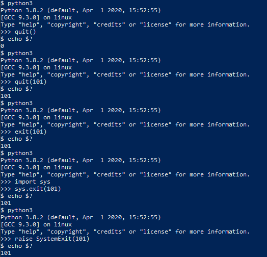
There are several ways to exit a Python Program that doesn’t involve throwing an exception, the first was going to try is quit()
You can use the bash command echo $? to get the exit code of the Python interpreter.
python3
Python 3.8.2 (default, Apr 1 2020, 15:52:55)
[GCC 9.3.0] on linux
Type "help", "copyright", "credits" or "license" for more information.
>>> quit()
$ echo $?
0
We can also define the type of code the interpreter should exit with by handing quit() an integer argument less than 256
python3
Python 3.8.2 (default, Apr 1 2020, 15:52:55)
[GCC 9.3.0] on linux
Type "help", "copyright", "credits" or "license" for more information.
>>> quit(101)
$ echo $?
101
exit() has the same functionality as it is an alias for quit()
python3
Python 3.8.2 (default, Apr 1 2020, 15:52:55)
[GCC 9.3.0] on linux
Type "help", "copyright", "credits" or "license" for more information.
>>> exit(101)
$ echo $?
101
Neither quit() nor exit() are considered good practice, as they both require the site module which is meant to be used for interactive interpreters and not in programs. For our programs, we should use something like sys.exit
python3
Python 3.8.2 (default, Apr 1 2020, 15:52:55)
[GCC 9.3.0] on linux
Type "help", "copyright", "credits" or "license" for more information.
>>> import sys
>>> sys.exit(101)
$ echo $?
101
Notice that we need to explicitly import a module to call exit(), this might seem like its not an improvement but it guarantees that the necessary module is loaded because it’s not a good assumption site will be loaded at runtime. If we don’t want to import extra modules, we can do what exit(), quit() and sys.exit() are doing behind the scenes and raise SystemExit
python3
Python 3.8.2 (default, Apr 1 2020, 15:52:55)
[GCC 9.3.0] on linux
Type "help", "copyright", "credits" or "license" for more information.
>>> raise SystemExit(101)
$ echo $?
101
Exit with error messages
What if we get bad input from a user? Let’s look back at our input.py script, and add the ability to handle bad input from the user (CTRL+D to pass an EOF character)
nano input.py
try:
name=input("What's your name?\n")
print("Hi, "+name+"!")
except EOFError:
print("EOFError: You didn't enter anything!")
$ python3 input.py
What's your name?
EOFError: You didn't enter anything!
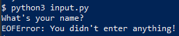
The try statement tells Python to try the code inside the statement and to pass any exception to the except statement before exiting.
Exiting without error
What if the user hands your program an error but you don’t want your code to print an error, or to do some sort of error handling to minimize user impact?
We can add a finally statement that lets us execute code after we do our error handling in catch
nano input.py
try:
name=input("What's your name?\n")
if(name==''):
print("Name cannot be blank!")
except EOFError:
#print("EOFError: You didn't enter anything!")
name="Blankname"
finally:
print("Hi, "+name+"!")
$ python3 input.py
What's your name?
Hi, Blankname!
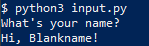
Notice the user would never know an EOFError occurred, this can be used to pass default values in the event of poor input or arguments.
Exit and release your resources
Generally, Python releases all the resources you’ve called in your program automatically when it exits, but for certain processes, it’s good practice to encase some limited resources in a with block.
Often you’ll see this in open() calls, where failing to properly release the file could cause problems with reading or writing to the file later.
nano openfile.py
with open("testfile.txt","w") as file:
file.write("let's write some text!\n")
$ python3 openfile.py
$ cat testfile.txt
let's write some text!
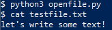
The with block automatically releases all resources requisitioned within it. If we wanted to more explicitly ensure the file was closed, we can use the atexit.register() command to call close()
$ nano openfile.py
import atexit
file=open("testfile.txt","w")
file.write("let's write some text!\n")
atexit.register(file.close)
If resources are called without using a with block, make sure to explicitly release them in an atexit command.
Exit after a time
If we are worried our program might never terminate normally, then we can use Python’s multiprocessing module to ensure our program will terminate.
$ nano waiting.py
import time
import sys
from multiprocessing import Process
integer=sys.argv[1]
init=map(int, integer.strip('[]'))
num=list(init)[0]
def exclaim(int):
time.sleep(int)
print("You were very patient!")
if __name__ == '__main__':
program = Process(target=exclaim, args=(num,))
program.start()
program.join(timeout=5)
program.terminate()
$ python3 waiting.py 7
$ python3 waiting.py 0
You were very patient!
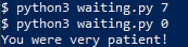
Notice how the process failed to complete when the function was told to wait for 7 seconds but completed and printed what it was supposed to when it was told to wait 0 seconds!
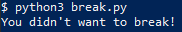
Exiting using a return statement
If we have a section of code we want to use to terminate the whole program, instead of letting the break statement continue code outside the loop, we can use the return sys.exit() to exit the code completely.
$ nano break.py
import time
import sys
def stop(isTrue):
for a in range(0,1):
if isTrue:
break
else:
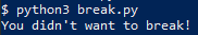
print("You didn't want to break!")
return sys.exit()
mybool = False
stop(mybool)
print("You used break!")
Exit in the middle of a function
If we don’t want to use a return statement, we can still call the sys.exit() to close our program and provide a return in another branch. Let’s use our code from break.py again.
$ nano break.py
import time
import sys
def stop(isTrue):
for a in range(0,1):
if isTrue:
word="bird"
break
else:
print("You didn't want to break!")
sys.exit()
mybool = False
print(stop(mybool))
Exit when conditions are met
If we have a loop in our Python code and we want to make sure the code can exit if it encounters a problem, we can use a flag that it can check to terminate the program.
$ nano break.py
import time
import sys
myflag=False
def stop(val):
global myflag
while 1==1:
val=val+1
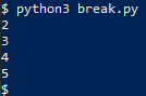
print(val)
if val%5==0:
myflag=True
if val%7==0:
myflag=True
if myflag:
sys.exit()
stop(1)
$ python3 break.py
2

3

4

5
Exit on keypress
If we want to hold our program open in the console till we press a key, we can use an unbound input() to close it.
$ nano holdopen.py
input("Press enter to continue")
$ python3 holdopen.py
Press enter to continue
$
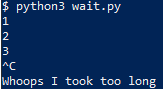
We can also pass CTRL+C to the console to give Python a KeyboardInterrupt character. We can even handle the KeyboardInterrupt exception like we’ve handled exceptions before.
$ nano wait.py
import time
try:
i=0
while 1==1:
i=i+1
print(i)
time.sleep(1)
except KeyboardInterrupt:
print("\nWhoops I took too long")
raise SystemExit
$ python3 wait.py
1

2

3

^C
Whoops I took too long
Exit a multithreaded program
Exiting a multithreaded program is slightly more involved, as a simple sys.exit() is called from the thread that will only exit the current thread. The “dirty” way to do it is to use os._exit()
$ nano threads.py
import threading
import os
import sys
import time
integer=sys.argv[1]
init=map(int, integer.strip('[]'))
num=list(init)[0]
def exclaim(int):
time.sleep(int)
os._exit(1)
print("You were very patient!")
if __name__ == '__main__':
program = threading.Thread(target=exclaim, args=(num,))
program.start()
program.join()
print("This should print before the main thread terminates!")
$ python3 threads.py 6
$
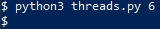
As you can see, the program didn’t print the rest of the program before it exited, this is why os._exit() is typically reserved for a last resort, and calling either Thread.join() from the main thread is the preferred method for ending a multithreaded program.
$ nano threads.py
import threading
import os
import sys
import time
import atexit
integer=sys.argv[1]
init=map(int, integer.strip('[]'))
num=list(init)[0]
atexit.register(print,"Threads exited successfully!")
def exclaim(int):
time.sleep(int)
print("You were very patient!")
if __name__ == '__main__':
program = threading.Thread(target=exclaim, args=(num,))
program.start()
program.join()
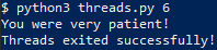
$ python3 threads.py 6
You were very patient!
Threads exited successfully!
End without sys exit
Sys.exit() is only one of several ways we can exit our python programs, what sys.exit() does is raise SystemExit, so we can just as easily use any built-in Python exception or create one of our own!
$ nano myexception.py
class MyException(Exception):
pass
try:
raise MyException()
except MyException:
print("The exception works!")
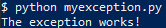
$ python3 myexception.py
The exception works!
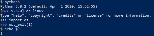
We can also use the os._exit() to tell the host system to kill the python process, although this doesn’t do atexit cleanup.
$ python3
Python 3.8.2 (default, Apr 1 2020, 15:52:55)
[GCC 9.3.0] on linux
Type "help", "copyright", "credits" or "license" for more information.
>>> import os
>>> os._exit(1)
Exit upon exception
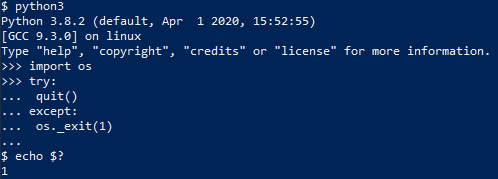
If we want to exit on any exception without any handling, we can use our try-except block to execute os._exit().
Note: this will also catch any sys.exit(), quit(), exit(), or raise SystemExit calls, as they all generate a SystemExit exception.
$ python3
Python 3.8.2 (default, Apr 1 2020, 15:52:55)
[GCC 9.3.0] on linux
Type "help", "copyright", "credits" or "license" for more information.
>>> import os
>>> try:
... quit()
... except:
... os._exit(1)
...
$ echo $?
1
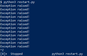
Exit and restart
Finally, we’ll explore what we do to exit Python and restart the program, which is useful in many cases.
$ nano restart.py
import atexit
import os
atexit.register(os.system,"python3 restart.py")
try:
n=0
while 1==1:
n=n+1
if n%5==0:
raise SystemExit
except:
print("Exception raised!")
$ python3 restart.py
Exception raised!
Exception raised!
...
Exception raised!
^Z
[3]+ Stopped python3 restart.py
I hope you find the tutorial useful. Keep coming back.
Thank you.


 C++, C, Java, Objective-C, Python, IDL, PHP, C#, Fortran, VHDL, Tcl ve bir dereceye kadar D dilleri için online/offline dokümantasyon hazırlamayı sağlayan bir dokümantasyon sistemi olan Doxygen‘in 1.8.19 sürümü duyuruldu. Deneysel çok iş parçacıklı girdi işleme desteği eklenen yeni sürüm, yüksek çözünürlüklü ekranlar için ölçeklenebilir arama çubuğu ile geliyor. Sqlite3 çıktısını daha iyi kontrol etmek için yapılandırma seçenekleri eklenen sürümde, Cmake’in ctest kullanarak testleri paralel olarak çalıştırması etkinleştirilmiş bulunuyor. Projelere ait dokümantasyon hazırlarken zaman bakımından büyük bir kazanç sağlayan yazılım, Mac OS X ve Linux altında geliştirilmiş, ancak oldukça taşınabilir bir platform olarak ayarlanmıştır. Doxygen ayrıca hepsi otomatik olarak üretilen bağımlılık grafiklerini, kalıtım şemalarını ve işbirliği şemalarını kullanarak çeşitli elemanlar arasındaki ilişkileri görselleştirebilir. Doxygen’i normal belgeler oluşturmak için de kullanabilirsiniz. Doxygen 1.8.19 hakkında ayrıntılı bilgi edinmek için değişiklikler sayfasını inceleyebilirsiniz.
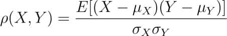
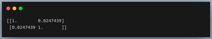
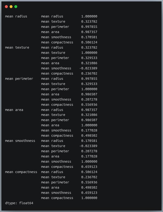
 In this blog, we will go through an important descriptive statistic of multi-variable data called the correlation matrix. We will learn how to create, plot, and manipulate correlation matrices in


 Debian
  Python ile yazılmış özgür, yüksek seviyeli,
  Today, we’ll be diving into the topic of exiting/terminating