
Linux çekirdeği resmi sitesi: https://www.kernel.org
Geliştirme & kararsız çekirdek:
5.7-rc5 2020-05-10
Linus Torvalds’ın duyurusu.
EndeavourOS 2020.05.08 duyuruldu
 Kolay kurulum ve önceden yapılandırılmış bir masaüstü ortamı sağlamayı hedefleyen Arch Linux tabanlı bir GNU/Linux dağıtımı olan EndeavourOS‘un 2020.05.08 sürümü duyuruldu. Bu sürümde, belirli donanım ve gerçek performanstaki bazı hatalarla ilgilenildiği belirtiliyor. 5.6.11 Linux çekirdeği üzerine yapılandırılan sistem, Firefox 76.0.1, Mesa 20.0.6 ve Calamares 3.2.20 gibi güncel paketler içeriyor. Önemli hata düzeltmeleriyle gelen sürümde, ATI/AMD ve Nvidia GPU’lar için önyükleme sorunlarının düzeltildiği söyleniyor. EndeavourOS 2020.05.08 hakkında ayrıntılı bilgi edinmek için sürüm duyurusunu inceleyebilirsiniz.
Debian Edu/Skolelinux Buster 10.4 çıktı
 Debian 10 “Buster”in dördüncü güvenlik ve hata düzeltme güncellemesi olarak Debian 10.4’ün 9 Mayıs 2020‘de duyurulmasının ardından, Debian Edu/Skolelinux Buster 10.4 de çıktı. Henüz resmi duyurusu yapılmamış olan sürüm, indirilmek üzere yansılarda yerini aldı. Yüzlerce paket ön yüklenmiş olarak gelen ve sonra da pek çok paketi ekleyebileceğiniz, Debian-edu projesince okullar ve üniversiteler için özel bir ortam sağlamayı hedefleyen ve özel bir Debian dağıtımı olarak geliştirilen Debian Edu/Skolelinux, okulda bir okul ağı mı, sunucular, iş istasyonları ve dizüstü bilgisayarlar mı kurulmak istendiğine veya Debian’ı ağ servisleriyle önceden yapılandırılmış olarak mı elde etmek istendiğine karar verilmesi suretiyle kullanılabiliyor. Ayrıca Skolelinux diye de adlandırılan Debian Edu, bilindiği gibi, okullar ve üniversiteler için özel bir ortam sağlamayı hedefleyen ve özel bir Debian dağıtımı olarak geliştirilen bir proje; sistemin, okullar ve üniversiteler için tam teşekküllü bir işletim sistemi olması arzu ediliyor.
Debian Edu okul sunucusu, bir LDAP veritabanı ve Kerberos kimlik doğrulama servisi, merkezi ev dizinleri, DHCP sunucusu, bir web proxy’si ve diğer birçok servis sağlar. Masaüstü 60’tan fazla eğitim yazılımı paketi içeriyor ve daha fazlası Debian arşivinden edinilebilir. Okullar masaüstü ortamları Xfce, GNOME, LXDE, MATE, KDE Plazma ve LXQt arasında seçim yapabilir. Debian Edu/Skolelinux Buster 10.4 edinmek için aşağıdaki linklerden yararlanabilirsiniz.
Debian’a LMDE nasıl eklenir?
 Bilindiği gibi, Debian Türkiye Forum’un değerli bir üyesi, değerli arkadaşımız Vedat Kılıç; uzun zamandır kendine özgü ISO kalıpları hazırlıyor. Vedat, bunları kendisine ait olan gnulinuxfree.blogspot.com üzerinden yayımlıyor. Bilindiği gibi, daha geniş bir çevreye duyurulması amacıyla bu çalışmaları forum üzerinden ve buradan da sizlere duyurmaya çaba gösteriyoruz. Vedat Kılıç‘ın en son yazdığı”Debian’a LMDE nasıl eklenir?” adlı yazıyla ilginç bir konuya değinmiş. Dostumuzun yazısını buraya aktarma gereği duyduk. Yazısına şu şekilde başlamış Vedat: “LMDE “Linux Mint Debian Edition” çoğumuzun bildiği gibi Debian Stable tabanlı bir dağıtımdır. Mint topluluğu bu dağıtım için bir çok yararlı yazılım geliştirmiş. Resimlerde göründüğü gibi bu yazılımlar bir çok işi kolaylaştıran, oldukça kullanışlı ve son kullanıcıyı hedef alarak geliştirilmiş. Debian’ı daha kullanışlı yapmak isteyenler için gerçekten güzel bir imkan. Üstelik kararlı olduğu için çakışma veya kaynak kullanımında artış olmaması onu daha cazip hale getiriyor. Debian’ın kullandığı sistem kaynağı ne ise LMDE’yi ekledikten sonra yine aynı kaynağı kullanıyor. LMDE sadece Cinnamon oturumu üzerine inşa edilmiş. Bu nedenle biz de kurulu sisteme LMDE’yi ekleyerek kendi masaüstümüzde onun araçlarından yararlanacağız.”
“Kendim Xfce ortamında denedim, diğer masaüstlerinde de sorun olacağını zanetmiyorum, çünkü araçlar genel anlamda geliştirilmiş. Örneğin kurduğum araçlar şunlardır: mintupdate, mintinstall, mintstick, mintsources, mint-update-info, mint-mirrors. Ayrıca kendim geliştirdiğim Debian tabanlı sürümlere doğrudan eklemeyeceğim ama ekleme seçeneği koyacağım, isteyen tek tıkla ekleyebilecek. Siz de Debian ortamı kullanıyorsanız ve LMDE’nin bu güzide araçlarından yararlanmak isterseniz işleme başlayalım. Önce alttaki LMDE 4 (Debbie) deposundan linuxmint-keyring paketini indirin.
LMDE Debbie
İndirdiğiniz deb formatlı paketi Gdebi kuruluysa sağ tık Gdebi seçeneğinden kurabilirsiniz. Komut ile kurmak isterseniz paketi indirdiğiniz dizinde uçbirimi açın ve alttaki komutu girin.”
sh -c "sudo dpkg -i *.deb ; echo 'y' | sudo apt install -f"
“Paket kurulduysa alttaki komutla LMDE deposunu gerekli dosyaya ekleyelim, komutu olduğu gibi uçbirime yapıştırın.”
sudo cat <> /etc/apt/sources.list
deb http://packages.linuxmint.com debbie main upstream import backport
EOF
“Ardından depo listesini güncelleyelim.”
sudo apt update
“Bu şekilde Debian ortamına LMDE eklemiş olduk, artık yukarıda sıraladığım paketleri veya başka tercihiniz olan LMDE araçlarını kurabilirsiniz. Ancak yukarıda sıraladığım paketler sistem paketleri olduğu için mutlaka kurmanızı öneririm, çok işinize yarayacaktır. Kurmak isterseniz alttaki komutu kullanabilirsiniz.”
sudo apt install mintupdate mintinstall mintstick mintsources mint-update-info mint-mirrors -y
“Bilgisayarı yeniden başlattıktan sonra kısmen melez sayılabilecek ve daha kullanışlı bir sisteminiz olur. Debian’a LMDE nasıl eklenir? işlemi burada bitti, kolay gelsin.
Güncelleme Yöneticisi, listeyi yeniler, temizler, güncelleme yapar, bildirimde bulunur ve hata olduğunda uyarı verir.”

“Yazılım Yöneticisi, paket arar, kurar, kaldırır, paketleri kategorilere ayırır, yazılımları logolarıyla gösterir, özet açıklamada bulunur ve kullanıcı yorumlarını okuma veya yorumda bulunma imkanı sunar.”

“Yazılım Kaynakları, Debian ve LMDE depolarının en hızlısını bulma ve seçme şansı verir.
Ayrıca anahtar aktarma gibi bir çok özelliği bulunuyor, bu araç favorim diyebilirim.”

Exiting/Terminating Python scripts (Simple Examples)
 Today, we’ll be diving into the topic of exiting/terminating Python scripts! Before we get started, you should have a basic understanding of what Python is and some basic knowledge about its use. You can use the IDE of your choice, but I’ll use Microsoft’s Linux Subsystem for Windows (WSL) package this time. For more information on that and how you enable it on Windows 10 go here. The way Python executes a code block makes it execute each line in order, checking dependencies to import, reading definitions and classes to store in memory, and executing pieces of code in order allowing for loops and calls back to the defined definitions and classes. When the Python interpreter reaches the end of the file (EOF), it notices that it can’t read any more data from the source, whether that be the user’s input through an IDE or reading from a file. To demonstrate let’s try to get user input and interrupt the interpreter in the middle of execution!
Why does Python automatically exit a script when it’s done?
First, from your bash terminal in your PowerShell open a new file called “input.py”
nano input.py
Then paste the following into the shell by right-clicking on the PowerShell window
name=input("Don't type anything!\n")
print("Hi,",name,"!")
Now, press CTRL+X to save and exit the nano window and in your shell type:
python3 input.py
Don't type anything!
And press CTRL+D to terminate the program while it’s waiting for user input
Traceback (most recent call last):
File "input.py", line 1, in
name=input("Don't type anything!")
EOFError
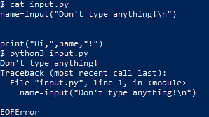
The EOFError exception tells us that the Python interpreter hit the end of file (EOF) condition before it finished executing the code, as the user entered no input data.
When Python reaches the EOF condition at the same time that it has executed all the code it exits without throwing any exceptions which is one way Python may exit “gracefully.”
Detect script exit
If we want to tell when a Python program exits without throwing an exception, we can use the built-in Python atexit module.
Theatexit handles anything we want the program to do when it exits and is typically used to do program clean up before the program process terminates
To experiment with atexit, let’s modify our input.py example to print a message at the program exit. Open the input.py file again and replace the text with this
import atexit
atexit.register(print,"Program exited successfully!")
name=input("What's your name?\n")
print("Hi,",name,"!")
Type your name and when you hit enter you should get:
What's your name?
Example
Hi, Example !
Program exited successfully!
Notice how the exit text appears at the end of the output no matter where we place the atexit call, and how if we replace the atexit call with a simple print(), we get the exit text where the print() all was made, rather than where the code exits.
Program exited successfully!
What's your name?
Example
Hi, Example !
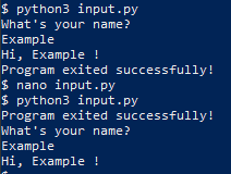
Graceful exit
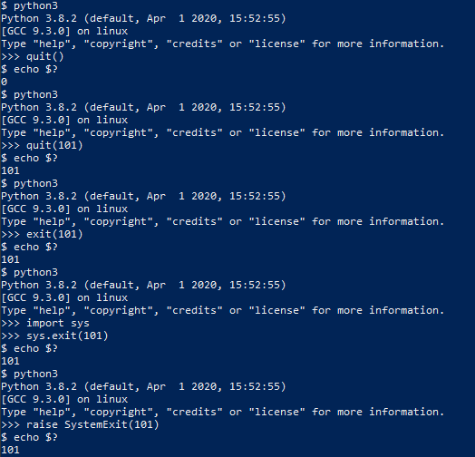
There are several ways to exit a Python Program that doesn’t involve throwing an exception, the first was going to try is quit()
You can use the bash command echo $? to get the exit code of the Python interpreter.
python3
Python 3.8.2 (default, Apr 1 2020, 15:52:55)
[GCC 9.3.0] on linux
Type "help", "copyright", "credits" or "license" for more information.
>>> quit()
$ echo $?
0
We can also define the type of code the interpreter should exit with by handing quit() an integer argument less than 256
python3
Python 3.8.2 (default, Apr 1 2020, 15:52:55)
[GCC 9.3.0] on linux
Type "help", "copyright", "credits" or "license" for more information.
>>> quit(101)
$ echo $?
101
exit() has the same functionality as it is an alias for quit()
python3
Python 3.8.2 (default, Apr 1 2020, 15:52:55)
[GCC 9.3.0] on linux
Type "help", "copyright", "credits" or "license" for more information.
>>> exit(101)
$ echo $?
101
Neither quit() nor exit() are considered good practice, as they both require the site module which is meant to be used for interactive interpreters and not in programs. For our programs, we should use something like sys.exit
python3
Python 3.8.2 (default, Apr 1 2020, 15:52:55)
[GCC 9.3.0] on linux
Type "help", "copyright", "credits" or "license" for more information.
>>> import sys
>>> sys.exit(101)
$ echo $?
101
Notice that we need to explicitly import a module to call exit(), this might seem like its not an improvement but it guarantees that the necessary module is loaded because it’s not a good assumption site will be loaded at runtime. If we don’t want to import extra modules, we can do what exit(), quit() and sys.exit() are doing behind the scenes and raise SystemExit
python3
Python 3.8.2 (default, Apr 1 2020, 15:52:55)
[GCC 9.3.0] on linux
Type "help", "copyright", "credits" or "license" for more information.
>>> raise SystemExit(101)
$ echo $?
101
Exit with error messages
What if we get bad input from a user? Let’s look back at our input.py script, and add the ability to handle bad input from the user (CTRL+D to pass an EOF character)
nano input.py
try:
name=input("What's your name?\n")
print("Hi, "+name+"!")
except EOFError:
print("EOFError: You didn't enter anything!")
$ python3 input.py
What's your name?
EOFError: You didn't enter anything!

The try statement tells Python to try the code inside the statement and to pass any exception to the except statement before exiting.
Exiting without error
What if the user hands your program an error but you don’t want your code to print an error, or to do some sort of error handling to minimize user impact?
We can add a finally statement that lets us execute code after we do our error handling in catch
nano input.py
try:
name=input("What's your name?\n")
if(name==''):
print("Name cannot be blank!")
except EOFError:
#print("EOFError: You didn't enter anything!")
name="Blankname"
finally:
print("Hi, "+name+"!")
$ python3 input.py
What's your name?
Hi, Blankname!
![]()
Notice the user would never know an EOFError occurred, this can be used to pass default values in the event of poor input or arguments.
Exit and release your resources
Generally, Python releases all the resources you’ve called in your program automatically when it exits, but for certain processes, it’s good practice to encase some limited resources in a with block.
Often you’ll see this in open() calls, where failing to properly release the file could cause problems with reading or writing to the file later.
nano openfile.py
with open("testfile.txt","w") as file:
file.write("let's write some text!\n")
$ python3 openfile.py
$ cat testfile.txt
let's write some text!
![]()
The with block automatically releases all resources requisitioned within it. If we wanted to more explicitly ensure the file was closed, we can use the atexit.register() command to call close()
$ nano openfile.py
import atexit
file=open("testfile.txt","w")
file.write("let's write some text!\n")
atexit.register(file.close)
If resources are called without using a with block, make sure to explicitly release them in an atexit command.
Exit after a time
If we are worried our program might never terminate normally, then we can use Python’s multiprocessing module to ensure our program will terminate.
$ nano waiting.py
import time
import sys
from multiprocessing import Process
integer=sys.argv[1]
init=map(int, integer.strip('[]'))
num=list(init)[0]
def exclaim(int):
time.sleep(int)
print("You were very patient!")
if __name__ == '__main__':
program = Process(target=exclaim, args=(num,))
program.start()
program.join(timeout=5)
program.terminate()
$ python3 waiting.py 7
$ python3 waiting.py 0
You were very patient!
![]()
Notice how the process failed to complete when the function was told to wait for 7 seconds but completed and printed what it was supposed to when it was told to wait 0 seconds!
Exiting using a return statement
If we have a section of code we want to use to terminate the whole program, instead of letting the break statement continue code outside the loop, we can use the return sys.exit() to exit the code completely.
$ nano break.py
import time
import sys
def stop(isTrue):
for a in range(0,1):
if isTrue:
break
else:
print("You didn't want to break!")
return sys.exit()
mybool = False
stop(mybool)
print("You used break!")
![]()
Exit in the middle of a function
If we don’t want to use a return statement, we can still call the sys.exit() to close our program and provide a return in another branch. Let’s use our code from break.py again.
$ nano break.py
import time
import sys
def stop(isTrue):
for a in range(0,1):
if isTrue:
word="bird"
break
else:
print("You didn't want to break!")
sys.exit()
mybool = False
print(stop(mybool))
![]()
Exit when conditions are met
If we have a loop in our Python code and we want to make sure the code can exit if it encounters a problem, we can use a flag that it can check to terminate the program.
$ nano break.py
import time
import sys
myflag=False
def stop(val):
global myflag
while 1==1:
val=val+1
print(val)
if val%5==0:
myflag=True
if val%7==0:
myflag=True
if myflag:
sys.exit()
stop(1)
$ python3 break.py
2

3

4

5

Exit on keypress
If we want to hold our program open in the console till we press a key, we can use an unbound input() to close it.
$ nano holdopen.py
input("Press enter to continue")
$ python3 holdopen.py
Press enter to continue
$
We can also pass CTRL+C to the console to give Python a KeyboardInterrupt character. We can even handle the KeyboardInterrupt exception like we’ve handled exceptions before.
$ nano wait.py
import time
try:
i=0
while 1==1:
i=i+1
print(i)
time.sleep(1)
except KeyboardInterrupt:
print("\nWhoops I took too long")
raise SystemExit
$ python3 wait.py
1

2

3

^C
Whoops I took too long

Exit a multithreaded program
Exiting a multithreaded program is slightly more involved, as a simple sys.exit() is called from the thread that will only exit the current thread. The “dirty” way to do it is to use os._exit()
$ nano threads.py
import threading
import os
import sys
import time
integer=sys.argv[1]
init=map(int, integer.strip('[]'))
num=list(init)[0]
def exclaim(int):
time.sleep(int)
os._exit(1)
print("You were very patient!")
if __name__ == '__main__':
program = threading.Thread(target=exclaim, args=(num,))
program.start()
program.join()
print("This should print before the main thread terminates!")
$ python3 threads.py 6
$
![]()
As you can see, the program didn’t print the rest of the program before it exited, this is why os._exit() is typically reserved for a last resort, and calling either Thread.join() from the main thread is the preferred method for ending a multithreaded program.
$ nano threads.py
import threading
import os
import sys
import time
import atexit
integer=sys.argv[1]
init=map(int, integer.strip('[]'))
num=list(init)[0]
atexit.register(print,"Threads exited successfully!")
def exclaim(int):
time.sleep(int)
print("You were very patient!")
if __name__ == '__main__':
program = threading.Thread(target=exclaim, args=(num,))
program.start()
program.join()
$ python3 threads.py 6
You were very patient!
Threads exited successfully!
![]()
End without sys exit
Sys.exit() is only one of several ways we can exit our python programs, what sys.exit() does is raise SystemExit, so we can just as easily use any built-in Python exception or create one of our own!
$ nano myexception.py
class MyException(Exception):
pass
try:
raise MyException()
except MyException:
print("The exception works!")
$ python3 myexception.py
The exception works!
![]()
We can also use the os._exit() to tell the host system to kill the python process, although this doesn’t do atexit cleanup.
$ python3
Python 3.8.2 (default, Apr 1 2020, 15:52:55)
[GCC 9.3.0] on linux
Type "help", "copyright", "credits" or "license" for more information.
>>> import os
>>> os._exit(1)

Exit upon exception
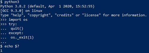
If we want to exit on any exception without any handling, we can use our try-except block to execute os._exit().
Note: this will also catch any sys.exit(), quit(), exit(), or raise SystemExit calls, as they all generate a SystemExit exception.
$ python3
Python 3.8.2 (default, Apr 1 2020, 15:52:55)
[GCC 9.3.0] on linux
Type "help", "copyright", "credits" or "license" for more information.
>>> import os
>>> try:
... quit()
... except:
... os._exit(1)
...
$ echo $?
1
Exit and restart
Finally, we’ll explore what we do to exit Python and restart the program, which is useful in many cases.
$ nano restart.py
import atexit
import os
atexit.register(os.system,"python3 restart.py")
try:
n=0
while 1==1:
n=n+1
if n%5==0:
raise SystemExit
except:
print("Exception raised!")
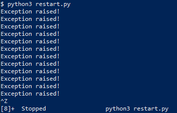
$ python3 restart.py
Exception raised!
Exception raised!
...
Exception raised!
^Z
[3]+ Stopped python3 restart.py
I hope you find the tutorial useful. Keep coming back.
Thank you.
20+ examples for NumPy matrix multiplication
 In this tutorial, we will look at various ways of performing matrix multiplication using NumPy arrays. we will learn how to multiply matrices with different sizes together. Also. we will learn how to speed up the multiplication process using GPU and other hot topics, so let’s get started! Before we move ahead, it is better to review some basic terminologies of Matrix Algebra. Basic Terminologies: Vector: Algebraically, a vector is a collection of coordinates of a point in space. Thus, a vector with 2 values represents a point in a 2-dimensional space. In Computer Science, a vector is an arrangement of numbers along a single dimension. It is also commonly known as an array or a list or a tuple. Eg. [1,2,3,4] Matrix: A matrix (plural matrices) is a 2-dimensional arrangement of numbers or a collection of vectors.
Ex:
[[1,2,3],
[4,5,6],
[7,8,9]]
Dot Product: A dot product is a mathematical operation between 2 equal-length vectors.
It is equal to the sum of the products of the corresponding elements of the vectors.

With a clear understanding of these terminologies, we are good to go.
Matrix multiplication with a vector
Let’s begin with a simple form of matrix multiplication – between a matrix and a vector.
Before we proceed, let’s first understand how a matrix is represented using NumPy.
NumPy’s array() method is used to represent vectors, matrices, and higher-dimensional tensors. Let’s define a 5-dimensional vector and a 3×3 matrix using NumPy.
import numpy as np
a = np.array([1, 3, 5, 7, 9])
b = np.array([[1, 2, 3],
[4, 5, 6],
[7, 8, 9]])
print("Vector a:\n", a)
print()
print("Matrix b:\n", b)
Output:
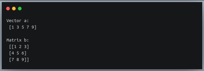
Let us now see how multiplication between a matrix and a vector takes place.
The following points should be kept in mind for a matrix-vector multiplication:
- The result of a matrix-vector multiplication is a vector.
- Each element of this vector is got by performing a dot product between each row of the matrix and the vector being multiplied.
- The number of columns in the matrix should be equal to the number of elements in the vector.

We’ll use NumPy’s matmul() method for most of our matrix multiplication operations.
Let’s define a 3×3 matrix and multiply it with a vector of length 3.
import numpy as np
a = np.array([[1, 2, 3],
[4, 5, 6],
[7, 8, 9]])
b= np.array([10, 20, 30])
print("A =", a)
print("b =", b)
print("Ab =",np.matmul(a,b))
Output:

Notice how the result is a vector of length equal to the rows of the multiplier matrix.
Multiplication with another matrix
Now, we understood the multiplication of a matrix with a vector, it would be easy to figure out the multiplication of two matrices.
But, before that, let’s review the most important rules of matrix multiplication:
- The number of columns in the first matrix should be equal to the number of rows in the second matrix.
- If we are multiplying a matrix of dimensions m x n with another matrix of dimensions n x p, then the resultant product will be a matrix of dimensions m x p.
Let us consider multiplication of an m x n matrix A with an n x p matrix B: 
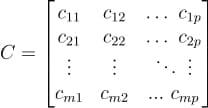
The product of the two matrices C = AB will have m row and p columns.
Each element in the product matrix C results from a dot product between a row vector in A and a column vector in B.

Let us now do a matrix multiplication of 2 matrices in Python, using NumPy.
We’ll randomly generate 2 matrices of dimensions 3 x 2 and 2 x 4.
We will use np.random.randint() method to generate the numbers.
import numpy as np
np.random.seed(42)
A = np.random.randint(0, 15, size=(3,2))
B = np.random.randint(0, 15, size =(2,4))
print("Matrix A:\n", A)
print("shape of A =", A.shape)
print()
print("Matrix B:\n", B)
print("shape of B =", B.shape)
Output:
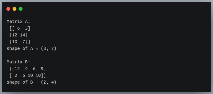
Note: we are setting a random seed using ‘np.random.seed()’ to make the random number generator deterministic.
This will generate the same random numbers each time you run this code snippet. This step is essential if you want to reproduce your result at a later point.
You can set any other integer as seed, but I suggest to set it to 42 for this tutorial so that your output will match the ones shown in the output screenshots.
Let us now multiply the two matrices using the np.matmul() method. The resulting matrix should have the shape 3 x 4.
C = np.matmul(A, B)
print("product of A and B:\n", C)
print("shape of product =", C.shape)
Output:

Multiplication between 3 matrices
Multiplication of the 3 matrices will be composed of two 2-matrix multiplication operations and each of the two operations will follow the same rules as discussed in the previous section.
Let us say we are multiplying 3 matrices A, B, and C; and the product is D = ABC.
Here, the number of columns in A should be equal to the number of rows in B and the number of rows in C should be equal to the number of columns in B.
The resulting matrix will have rows equal to the number of rows in A, and columns equal to the number of columns in C.
An important property of matrix multiplication operation is that it is Associative.
With multi-matrix multiplication, the order of individual multiplication operations does not matter and hence does not yield different results.
For instance, in our example of multiplication of 3 matrices D = ABC, it doesn’t matter if we perform AB first or BC first.

Both orderings would yield the same result. Let us do an example in Python.
import numpy as np
np.random.seed(42)
A = np.random.randint(0, 10, size=(2,2))
B = np.random.randint(0, 10, size=(2,3))
C = np.random.randint(0, 10, size=(3,3))
print("Matrix A:\n{}, shape={}\n".format(A, A.shape))
print("Matrix B:\n{}, shape={}\n".format(B, B.shape))
print("Matrix C:\n{}, shape={}\n".format(C, C.shape))
Output:
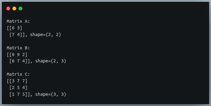
Based on the rules we discussed above, the multiplication of these 3 matrices should yield a resulting matrix of shape (2, 3).
Note that the method np.matmul() accepts only 2 matrices as input for multiplication, so we will call the method twice in the order that we wish to multiply, and pass the result of the first call as a parameter to the second.
(We’ll find a better way to deal with this problem in a later section when we introduce ‘@’ operator)
Let’s do the multiplication in both orders and validate the property of associativity.
D = np.matmul(np.matmul(A,B), C)
print("Result of multiplication in the order (AB)C:\n\n{},shape={}\n".format(D, D.shape))
D = np.matmul(A, np.matmul(B,C))
print("Result of multiplication in the order A(BC):\n\n{},shape={}".format(D, D.shape))
Output:
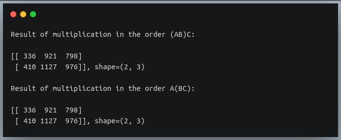
As we can see, the result of multiplication of the 3 matrices remains the same whether we multiply A and B first, or B and C first.
Thus, the property of associativity stands validated.
Also, the shape of the resulting array is (2, 3) which is on the expected lines.
NumPy 3D matrix multiplication
A 3D matrix is nothing but a collection (or a stack) of many 2D matrices, just like how a 2D matrix is a collection/stack of many 1D vectors.
So, matrix multiplication of 3D matrices involves multiple multiplications of 2D matrices, which eventually boils down to a dot product between their row/column vectors.
Let us consider an example matrix A of shape (3,3,2) multiplied with another 3D matrix B of shape (3,2,4).
import numpy as np
np.random.seed(42)
A = np.random.randint(0, 10, size=(3,3,2))
B = np.random.randint(0, 10, size=(3,2,4))
print("A:\n{}, shape={}\nB:\n{}, shape={}".format(A, A.shape,B, B.shape))
Output:
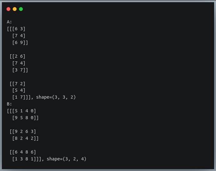
The first matrix is a stack of three 2D matrices each of shape (3,2) and the second matrix is a stack of 3 2D matrices, each of shape (2,4).
The matrix multiplication between these two will involve 3 multiplications between corresponding 2D matrices of A and B having shapes (3,2) and (2,4) respectively.
Specifically, the first multiplication will be between A[0] and B[0], the second multiplication will be between A[1] and B[1] and finally, the third multiplication will be between A[2] and B[2].
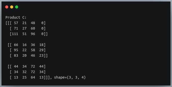
The result of each individual multiplication of 2D matrices will be of shape (3,4). Hence, the final product of the two 3D matrices will be a matrix of shape (3,3,4).
Let’s realize this using code.
C = np.matmul(A,B)
print("Product C:\n{}, shape={}".format(C, C.shape))
Output:
Alternatives to np.matmul()
Apart from ‘np.matmul()’, there are two other ways of doing matrix multiplication – the np.dot() method and the ‘@’ operator, each offering some differences/flexibility in matrix multiplication operations.
The ‘np.dot()’ method
This method is primarily used to find the dot product of vectors, but if we pass two 2-D matrices, then it will behave similarly to the ‘np.matmul()’ method and will return the result of the matrix multiplication of the two matrices.
Let us look at an example:
import numpy as np
# a 3x2 matrix
A = np.array([[8, 2, 2],
[1, 0, 3]])
# a 2x3 matrix
B = np.array([[1, 3],
[5, 0],
[9, 6]])
# dot product should return a 2x2 product
C = np.dot(A, B)
print("product of A and B:\n{} shape={}".format(C, C.shape))
Output:

Here, we defined a 3×2 matrix and a 2×3 matrix and their dot product yields a 2×2 result which is the matrix multiplication of the two matrices,
the same as what ‘np.matmul()’ would have returned.
The difference between np.dot() and np.matmul() is in their operation on 3D matrices.
While ‘np.matmul()’ operates on two 3D matrices by computing matrix multiplication of the corresponding pairs of 2D matrices (as discussed in the last section), np.dot() on the other hand computes dot products of various pairs of row vectors and column vectors from the first and second matrix respectively.
np.dot() on two 3D matrices A and B returns a sum-product over the last axis of A and the second-to-last axis of B.
This is non-intuitive, and not easily comprehensible.
So, if A is of shape (a, b, c) and B is of shape (d, c, e), then the result of np.dot(A, B) will be of shape (a,d,b,e) whose individual element at a position (i,j,k,m) is given by:
dot(A, B)[i,j,k,m] = sum(A[i,j,:] * B[k,:,m])
Let’s check an example:
import numpy as np
np.random.seed(42)
A = np.random.randint(0, 10, size=(2,3,2))
B = np.random.randint(0, 10, size=(3,2,4))
print("A:\n{}, shape={}\nB:\n{}, shape={}".format(A, A.shape,B, B.shape))
Output:
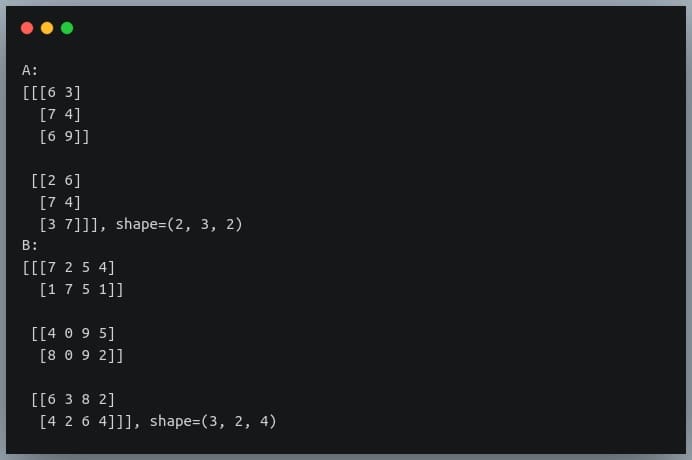
If we now pass these matrices to the ‘np.dot()’ method, it will return a matrix of shape (2,3,3,4) whose individual elements are computed using the formula given above.
C = np.dot(A,B)
print("np.dot(A,B) =\n{}, shape={}".format(C, C.shape))
Output:
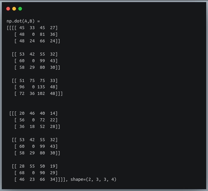
Another important difference between ‘np.matmul()’ and ‘np.dot()’ is that ‘np.matmul()’ doesn’t allow multiplication with a scalar (will be discussed in the next section), while ‘np.dot()’ allows it.
The ‘@’ operator
The @ operator introduced in Python 3.5, it performs the same operation as ‘np.matmul()’.
Let’s run through an earlier example of ‘np.matmul()’ using @ operator, and will see the same result as returned earlier:
import numpy as np
np.random.seed(42)
A = np.random.randint(0, 15, size=(3,2))
B = np.random.randint(0, 15, size =(2,4))
print("Matrix A:\n{}, shape={}".format(A, A.shape))
print("Matrix B:\n{}, shape={}".format(B, B.shape))
C = A @ B
print("product of A and B:\n{}, shape={}".format(C, C.shape))
Output:
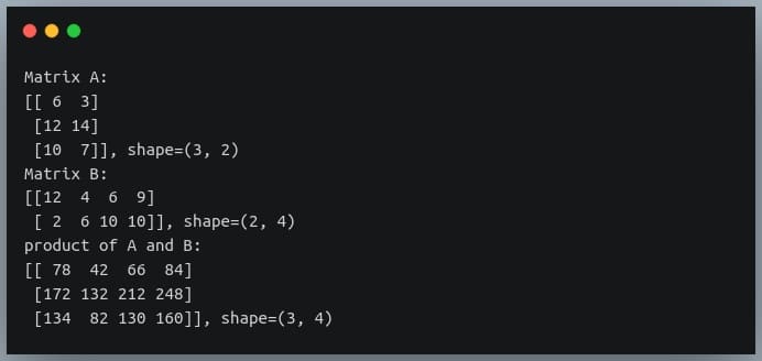
The ‘@’ operator becomes handy when we are performing matrix multiplication of over 2 matrices.
Earlier, we had to call ‘np.matmul()’ multiple times and pass their results as a parameter to the next call.
Now, we can perform the same operation in a simpler (and a more intuitive) way:
import numpy as np
np.random.seed(42)
A = np.random.randint(0, 10, size=(2,2))
B = np.random.randint(0, 10, size=(2,3))
C = np.random.randint(0, 10, size=(3,3))
print("Matrix A:\n{}, shape={}\n".format(A, A.shape))
print("Matrix B:\n{}, shape={}\n".format(B, B.shape))
print("Matrix C:\n{}, shape={}\n".format(C, C.shape))
D = A @ B @ C # earlier np.matmul(np.matmul(A,B),C)
print("Product ABC:\n\n{}, shape={}\n".format(D, D.shape))
Output:
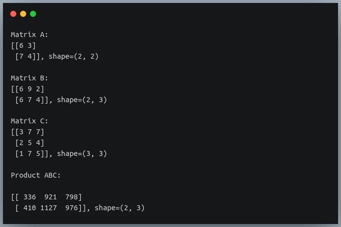
Multiplication with a scalar (Single value)
So far we’ve performed multiplication of a matrix with a vector or another matrix. But what happens when we perform matrix multiplication with a scalar or a single numeric value?
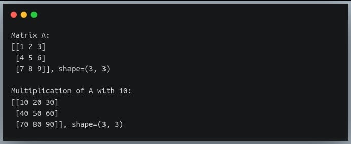
The result of such an operation is got by multiplying each element in the matrix with the scalar value. Thus the output matrix has the same dimension as the input matrix.
Note that ‘np.matmul()’ does not allow the multiplication of a matrix with a scalar. This can be achieved by using the np.dot() method or using the ‘*’ operator.
Let’s see this in a code example.
import numpy as np
A = np.array([[1,2,3],
[4,5, 6],
[7, 8, 9]])
B = A * 10
print("Matrix A:\n{}, shape={}\n".format(A, A.shape))
print("Multiplication of A with 10:\n{}, shape={}".format(B, B.shape))
Output:
Element-wise matrix multiplication
Sometimes we want to do multiplication of corresponding elements of two matrices having the same shape.

This operation is also called as the Hadamard Product. It accepts two matrices of the same dimensions and produces a third matrix of the same dimension.
It can be achieved in Python by calling the NumPy’s multiply() function or using the ‘*’ operator.
import numpy as np
np.random.seed(42)
A = np.random.randint(0, 10, size=(3,3))
B = np.random.randint(0, 10, size=(3,3))
print("Matrix A:\n{}\n".format(A))
print("Matrix B:\n{}\n".format(B))
C = np.multiply(A,B) # or A * B
print("Element-wise multiplication of A and B:\n{}".format(C))
Output:
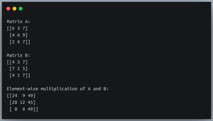
The only rule to be kept in mind for element-wise multiplication is that the two matrices should have the same shape.
However, if one dimension of a matrix is missing, NumPy would broadcast it to match the shape of the other matrix.
In fact, matrix multiplication with a scalar also involves the broadcasting of the scalar value to a matrix of the shape equal to the matrix operand in the multiplication.
That means when we are multiplying a matrix of shape (3,3) with a scalar value 10, NumPy would create another matrix of shape (3,3) with constant values 10 at all positions in the matrix and perform element-wise multiplication between the two matrices.
Let’s understand this through an example:
import numpy as np
np.random.seed(42)
A = np.random.randint(0, 10, size=(3,4))
B = np.array([[1,2,3,4]])
print("Matrix A:\n{}, shape={}\n".format(A, A.shape))
print("Matrix B:\n{}, shape={}\n".format(B, B.shape))
C = A * B
print("Element-wise multiplication of A and B:\n{}".format(C))
Output:
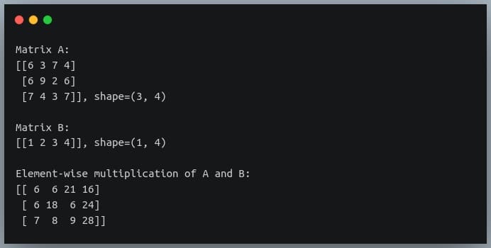
Notice how the second matrix which had shape (1,4) was transformed into a (3,4) matrix through broadcasting and the element-wise multiplication between the two matrices took place.
Matrix raised to a power (Matrix exponentiation)
Just like how we can raise a scalar value to an exponent, we can do the same operation with matrices.
Just as raising a scalar value (base) to an exponent n is equal to repeatedly multiplying the n bases, the same pattern is observed in raising a matrix to power, which involves repeated matrix multiplications.
For instance, if we raise a matrix A to a power n, it is equal to the matrix multiplications of n matrices, all of which will be the matrix A.

Note that for this operation to be possible, the base matrix has to be square.
This is to ensure the rules of matrix multiplication are followed (number of columns in preceding matrix = number of rows in the next matrix)
This operation is provided in Python by NumPy’s linalg.matrix_power() method, which accepts the base matrix and an integer power as its parameters.
Let us look at an example in Python:
import numpy as np
np.random.seed(10)
A = np.random.randint(0, 10, size=(3,3))
A_to_power_3 = np.linalg.matrix_power(A, 3)
print("Matrix A:\n{}, shape={}\n".format(A, A.shape))
print("A to the power 3:\n{}, shape={}".format(A_to_power_3,A_to_power_3.shape))
Output:
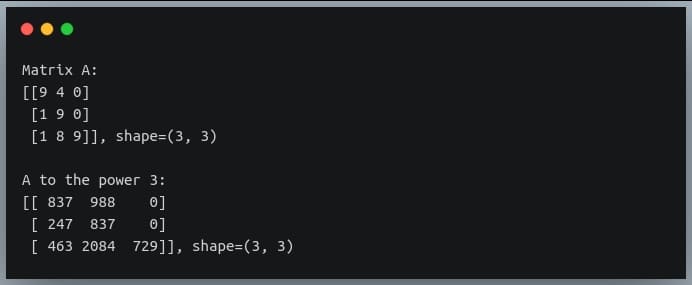
We can validate this result by doing normal matrix multiplication with 3 operands (all of them A), using the ‘@’ operator:
B = A @ A @ A
print("B = A @ A @ A :\n{}, shape={}".format(B, B.shape))
Output:

As you can see, the results from both operations are matching.
An important question that arises from this operation is – What happens when the power is 0?
To answer this question, let us review what happens when we raise a scalar base to power 0.
We get the value 1, right? Now, what is the equivalent of 1 in Matrix Algebra? You guessed it right!
It’s the identity matrix.
So raising an n x n matrix to the power 0 results in an identity matrix I of shape n x n.
Let’s quickly check this in Python, using our previous matrix A.
C = np.linalg.matrix_power(A, 0)
print("A to power 0:\n{}, shape={}".format(C, C.shape))
Output:

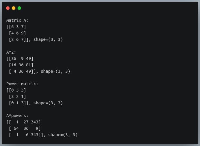
Element-wise exponentiation
Just like how we could do element-wise multiplication of matrices, we can also do element-wise exponentiation i.e. raise each individual element of a matrix to some power.
This can be achieved in Python using standard exponent operator ‘**‘ – an example of operator overloading.
Again, we can provide a single constant power for all the elements in the matrix, or a matrix of powers for each element in the base matrix.
Let’s look at examples of both in Python:
import numpy as np
np.random.seed(42)
A = np.random.randint(0, 10, size=(3,3))
print("Matrix A:\n{}, shape={}\n".format(A, A.shape))
#constant power
B = A**2
print("A^2:\n{}, shape={}\n".format(B, B.shape))
powers = np.random.randint(0, 4, size=(3,3))
print("Power matrix:\n{}, shape={}\n".format(powers, powers.shape))
C = A ** powers
print("A^powers:\n{}, shape={}\n".format(C, C.shape))
Output:
Multiplication from a particular index
Suppose we have a 5 x 6 matrix A and another 3 x 3 matrix B. Obviously, we cannot multiply these two together, because of dimensional inconsistencies.
But what if we wanted to multiply a 3×3 submatrix in matrix A with matrix B while keeping the other elements in A unchanged?
For better understanding, refer to the following image:

This operation can be achieved in Python, by using matrix slicing to extract the submatrix from A, performing multiplication with B, and then writing back the result at relevant index in A.
Let’s see this in action.
import numpy as np
np.random.seed(42)
A = np.random.randint(0, 10, size=(5,6))
B = np.random.randint(0, 10, size=(3,3))
print("Matrix A:\n{}, shape={}\n".format(A, A.shape))
print("Matrix B:\n{}, shape={}\n".format(B, B.shape))
C = A[1:4,2:5] @ B
A[1:4,2:5] = C
print("Matrix A after submatrix multiplication:\n{}, shape={}\n".format(A, A.shape))
Output:
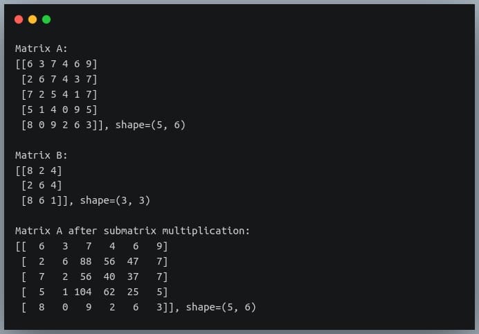
As you can see, only the elements at row indices 1 to 3 and column indices 2 to 4 have been multiplied with B and the same have been written back in A, while the remaining elements of A have remained unchanged.
Also, it’s unnecessary to overwrite the original matrix. We can also write the result in a new matrix, by first copying the original matrix to a new matrix and then writing the product at the position of the submatrix.
Matrix multiplication using GPU
We know that NumPy speeds up the matrix operations by parallelizing a lot of computations and making use of our CPU’s parallel computing capabilities.
However, modern-day applications need more than that. CPUs offer limited computation capabilities, and it does not suffice for the large number of computations that we need, typically in applications like deep learning.
That is where GPUs come into the picture. They offer large computation capabilities and excellent parallelized computation infrastructure, which helps us save a significant amount of time by doing hundreds of thousands of operations within fractions of seconds.
In this section, we will look at how we can perform matrix multiplication on a GPU, instead of a CPU and save a lot of time doing so.
NumPy does not offer the functionality to do matrix multiplications on GPU. So we must install some additional libraries that help us achieve our goal.
We will first install the ‘scikit-cuda‘ and ‘PyCUDA‘ libraries using pip install. These libraries help us perform computations on CUDA based GPUs. To install these libraries from your terminal, if you have a GPU installed on your machine.
pip install pycuda
pip install scikit-cuda
If you do not have a GPU on your machine, you can try out Google Colab notebooks, and enable GPU access, it’s free for use. Now we will write the code to generate two 1000×1000 matrices and perform matrix multiplication between them using two methods:
- Using NumPy’s ‘matmul()‘ method on a CPU
- Using scikit-cuda’s ‘linalg.mdot()‘ method on a GPU
In the second method, we will generate the matrices on a CPU, then we will store them on GPU (using PyCUDA’s ‘gpuarray.to_gpu()‘ method) before performing the multiplication between them. We will use the ‘time‘ module to compute the time of computation in both cases.
Using CPU
import numpy as np
import time
# generating 1000 x 1000 matrices
np.random.seed(42)
x = np.random.randint(0,256, size=(1000,1000)).astype("float64")
y = np.random.randint(0,256, size=(1000,1000)).astype("float64")
#computing multiplication time on CPU
tic = time.time()
z = np.matmul(x,y)
toc = time.time()
time_taken = toc - tic #time in s
print("Time taken on CPU (in ms) = {}".format(time_taken*1000))
Output:

On some old hardware systems, you may get a memory error, but if you are lucky, it will work in a long time (depends on your system).
Now, let us perform the same multiplication on a GPU and see how the time of computation differs between the two.
Using GPU
#computing multiplication time on GPU
linalg.init()
# storing the arrays on GPU
x_gpu = gpuarray.to_gpu(x)
y_gpu = gpuarray.to_gpu(y)
tic = time.time()
#performing the multiplication
z_gpu = linalg.mdot(x_gpu, y_gpu)
toc = time.time()
time_taken = toc - tic #time in s
print("Time taken on a GPU (in ms) = {}".format(time_taken*1000))
Output:

As we can see, performing the same operation on a GPU gives us a speed-up of 70 times as on CPU.
This was still a small computation. For large scale computations, GPUs give us speed-ups of a few orders of magnitude.
Conclusion
In this tutorial, we looked at how multiplication of two matrices takes place, the rules governing them, and how to implement them in Python.
We also looked at different variants of the standard matrix multiplication (and their implementation in NumPy) like multiplication of over 2 matrices, multiplication only at a particular index, or power of a matrix.
We also looked at element-wise computations in matrices such as element-wise matrix multiplication, or element-wise exponentiation.
Finally, we looked at how we can speed up the matrix multiplication process by performing them on a GPU.
Five Things You Must Consider Before ‘Developing an App’
 Before you begin developing an app, it is worth taking the time to properly plan out your development cycle. From defining your intended feature set to load testing, the more work you do before you start coding, the quicker you will be able to progress through the actual development of your app.Below are five essential things to consider before developing your app. The more detailed your initial plans for your app, the smoother the entire development process will go. Before you even think about how to actually code your app, you need to establish exactly what it is going to do and why it is going to be doing it. If you want to develop an app just for the sake of it, this is a great way to teach yourself new skills. But if you are looking at developing an app with an eye to commercializing it, you need to know exactly what you are doing before you begin.
The Purpose Of Your App
When developing an app for your business, there should be a clear rationale for you doing so. If you are only developing an app because you feel like you are supposed to or because your competitors have beaten you to the punch, the result is almost definitely going to be underwhelming.
On the other hand, if you take the time beforehand to plan your app properly and seriously consider how you can provide real value to your users, you stand a much better chance of critical and commercial success.
Before you can make any detailed plans about what your app will look like and what it will do, you need to be clear with yourself about what its main purpose is.
The Intended Feature Set
Once you have defined the ultimate purpose of your app, you can then begin to think about what features you need to include to achieve it.
Laying out your feature set should be one of the first things you do when you are preparing to develop an app. The features you want to include will have an impact on every other part of the design process.
For example, when it comes to your user interface, you will want to choose something that makes it easy for a user to see and access all of the features your app offers.
Equally, when you are assigning coders to various tasks, knowing what features you are shooting for will enable you to delegate work appropriately. There is no sense in asking a coder to work on a feature that lies well outside of their skill set.
The Price Point
If you are developing an app for a business, most of the time it will be distributed for free. It is important to know upfront whether the app you are working on is going to be provided for free, whether it will cost money, or whether there is an associated subscription cost as the buyer want to save money in all cases.
The price point at which you intend to sell an app will determine how much money you can sink into its development. It will also have a significant impact on the way that the app is marketed.
Fortunately, it is possible for you to have the best of all worlds when it comes to pricing. Many app developers have realized the potential in offering a free version of the app that is funded through advertising alongside a premium version that includes no ads.
The Platform
Before you can properly plan out your app development, you need to establish exactly what platform you are going to be aiming for.
Even if you intend to make your app available on every mobile operating system possible, you will still need to prioritize. In the vast majority of cases, it will make more sense to build your app for one primary platform first and then go about converting it for other platforms.
If you are trying to develop an app for multiple different platforms simultaneously, you are much more likely to run into problems.
Not only this, but you will find yourself having to solve problems for multiple different platforms at once. It is far more efficient to develop for your primary platform and iron out all the kinks before moving on to the next one.
App Load Testing
Developing an app is much more involved than many people realize. Lots of people think that once you have written the code and compiled the binary, your app is done and dusted. On the contrary, it doesn’t matter how talented your coders are or how much regression testing you have undertaken, there is still a range of things that you need to test under specific circumstances.
Load testing is one of many tests that can be used to assess an app’s performance under certain circumstances. Specifically, load testing will tell you how well your app performs when the system running it is under a heavy load and most of its available resources are being used.
For an app that is entirely offline, it is the system resources of the device it is running on that matter.
However, if your app also has online features, the current load placed on your internet connection will also be a factor in determining performance. In this case, many developers use proxies to load test their servers. Some proxy providers offer easy to use options.
Planning is everything in app development. If you take the time beforehand to work out exactly what you are doing and why then you will find the whole process much easier.


